In Neuroscience there exists what is known as The Cocktail Party Effect. When one is in a crowded environment, such as a cocktail party, despite the noisy environment they are able to focus their attention on a single speaker. This effect is often taken for granted as it occurs subconsciously, yet without it our hearing would be all but useless. As computers are applied in more and more social settings, an implementation of the cocktail party effect will be required to make sense of the noise around them. Completely replicating the effect is a large goal, but it is something that can be done in parts. Here I will take a first step by implementing an algorithm to determine the direction of the dominate sound source.

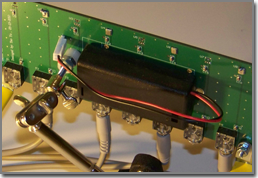
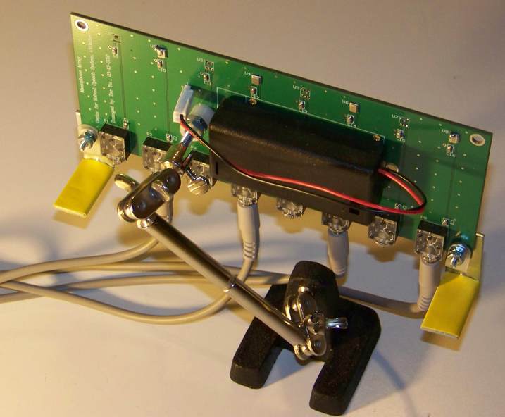
    The implementation which follows is based on this paper Blind Acoustic Beam-forming Based on Generalized Eigenvalue Decomposition. For this implementation we are using a 4 channel MEMS microphone array, hooked up to a TASCAM US-1641 ADC.

    We hope to find the direction of arrival (DoA) of the dominate sound, in our case we are focusing on human speech. To do this, we will want to collect samples and perform a Fourier Transform to get the frequencies of the noise recorded. The noise you hear is a very complex sound wave. A Fourier Transform will take that complex wave and split it into the individual component waves which add to form it.

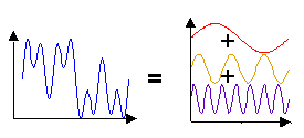
A complex wave is the sum of the
components.

The amplitude and frequency of
component waves.

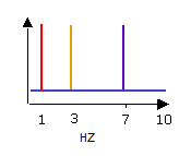
    This is called transforming into the frequency domain, where you have the frequencies of the individual waves which make up a more complex one. Human speech generally falls between 1000-2000 HZ, so once we are in the frequency domain we will discard everything outside that range. The result of a Fast Fourier Transform (FFT) is an array of complex numbers (a+bi) representing the amplitude and phase for each frequency.

    Before we do the FFT, we will want to normalize the signal at each microphone. To do this we will convert the signal to the number of standard deviations it is from the mean. We will need to first calculate the mean and standard deviation across each microphone. (See the Mean and Std notes on calculating running estimates for real-time applications.) Once we have that, to normalize we will take each sample, subtract the mean from it, and divide by the standard deviation. We calculate the normalized value for the k^th sample from the i^th microphone as


Now that we have our samples normalized, the first step is to perform the FFT.

Mic 0	S0,0	S0,1	S0,2	...	S0,255		a0,0 + b0,0i	a0,1 + b0,1i	...	a0,255 + b0,255i
Mic 1	S1,0	S1,1	S1,2	...	S1,255	FFT	a1,0 + b1,0i	a1,1 + b1,1i	...	a1,255 + b1,255i
Mic 2	S2,0	S2,1	S2,2	...	S2,255	==>	a2,0 + b2,0i	a2,1 + b2,1i	...	a2,255 + b2,255i
Mic 3	S3,0	S3,1	S3,2	...	S3,255		a3,0 + b3,0i	a3,1 + b3,1i	...	a3,255 + b3,255i
	For each microphone we take a track of 256 samples. Si,j is the jth normalized sample from the ith microphone						The FFT results in complex values where ai,j+bi,ji represents the amplitude and phase of sound in the jth frequency band from the ith microphone. Since we are working with 256 discrete values and not a continuous function, we end up with 256 discrete frequency bands

    Imagine a single sound wave moving across the room. As this wave propagates, it will strike 4 microphones at different times. The exact timing differences would depend on the frequency of the wave, and the direction it is traveling. Suppose we know the DoA of a wave at the first microphone, we should then be able to calculate when it hits the other microphones. This transfer function is known as the steering vectors; we will use . After calculating expected values for the other microphones we can compare those values to the actual values. This value represents the distortion of the signal across the microphones. We call this distortion the Spatial Response (SR). In an ideal setting, with no noise or echo, we could perfectly calculate the changes and we would expect the SR to be larger. We will use the SR to find the DoA. To do this we will calculate the SR for several directions, and choose the direction with the largest value.

    There are a few steps in calculating the SR. First, we will be working with the Cross Power Spectral Density (PSD) matrices of the microphone signal. While the name is a mouthful, it is not complicated. For a given frequency k, we will take the FFT result of that frequency from each of the 4 microphones and put them into a 4x1 matrix, we will call this matrix . Given a matrix of complex numbers, its Hermitian Transpose is found by transposing the matrix, and then flipping the sign of the imaginary component of each number. We denote the Hermition Transpose of as . The PSD matrix is defined as:
which is a 4x4 complex matrix.

=

a0,k + b0,ki

a1,k + b1,ki

a2,k + b2,ki

a3,k + b3,ki

=

C0

C1

C2

C3

	a0,k - b0,ki		C0H
=	a1,k - b1,ki	=	C1H
	a2,k - b2,ki		C2H
	a3,k - b3,ki		C3H

	C0HC0	C0HC1	C0HC2	C0HC3
=	C1HC0	C1HC1	C1HC2	C1HC3
	C2HC0	C2HC1	C2HC2	C2HC3
	C3HC0	C3HC1	C3HC2	C3HC3

    We can say that the microphone input is made of two components, the signal and noise. We are only interested in the signal, and would like to filter out as much noise as possible before performing the localization. We want to find a filter which will maximize the signal-to-noise ratio .
.

    We are interested in this filter because it is needed to calculate the SR. Later we can apply this filter to the microphone input to reduce the noise, but for now we are using it so we localize the dominate source and not noise. Along with the filter, we need . We will define the Spatial Response formally:



    We need to find and . The steering vectors, , is well known and defined as:

Let , and , where C = the speed of sound, and r = the distance between microphones.



is found to be the largest eigenvector of .

    Which leaves us in need of the PSD matrix for the noise, . To approximate this we can average the PSD matrices of the room's ambient noise over a few seconds. When approximating the noise, we will want to ensure that nobody is speaking loudly and we are only recording the background noise of the environment.

    With , , and , we are at last able to find .

    To get the direction of the dominate sound, we use by calculating the value for for each frequency at each direction. For each frequency we say the DoA is the theta which produces the largest value.
    When we actually localize, we will want to look at the dominate sound over a period of time. We are using an FFT length of 256, and a sample rate of 8000HZ, so each PSD matrix corresponds to a 0.032 second window. To prevent a short burst of noise from dominating the signal, and to reduce the computational load, we will average every 30 PSD matrices. This way we are localizing over a 1 second window.

    In summary, we were able to take samples from an array of microphones and estimate the direction of the dominate speech source. We accomplished this by first transforming the microphone values to cross-power spectral density matrix for each frequency band. Then we estimate the noise matrix by avergaing the PSD matrices across a few seconds. To localize, we take average the PSD matrices over 1 second as our PSD sample. For each frequency, we find the inverse noise matrix and multiply it by this PSD sample, then take the principal eigenvector of the resultign matrix. This is the filter to maximize the signal-to-noise ratio for a given frequency. Then we iteratate through directions and calculate the spatial response for each direction. The direction for each frequency is the direction which yields the highest spatial response. Our estimate for the direction of the dominate sound is the mean of the direction for each frequency.

    Of course this is only the start of things. The next step would be to use what we found to actually filter the noise and focus on the signal from a given source. Another research topic is multidiminsional arrays for multidiminsisional localization. One weakness of the approach outlined is that it attempts to correct for noise, but does nothing for echo. There is research in applying machine learning techniques to create predictive filters to account for noise and echo. Lastly, we are focusing on a single source, it would be useful separate and clean sounds from multiple sources.

C++ Implementation

You can find my implementation of this algorithm in Visual C++ here. It will find the direction of sound from a multi-channel wav file.
This depends on libSndFile for reading from wav files, and IT++ for FFT and matrix operations.
IT++ requires some underlying math libraries. I am using ACML.
Once the required libraries are installed, you will need to update the include and linker paths for the project to point to the correct locations.

Calculatind the Mean and Std

The mean and std are normally defined as:
, and
This is easy calculate if we are working with audio files where we have all future samples available. If we are working in real-time directly from microphones things are not as simple. What we will do is keep a running calculation of the mean and std. As we get new samples we will recalculate the values, but we need to do so in a time and memory effecient manner. Will we keep three totals where

Using those values we can calculate the mean and std as follows:

, and